Testing Menura against ion acoustic wave Landau damping
Commit a460d129
A quasi-1-dimensional box is initialised with a density profile taken as 5 spatial periods of a sinus, of amplitude 0.05 of the average density.
[1]:
from menura_utils import *
import own_tools as oT
import own_colours as oC
path = '../menura'
[2]:
mp = menura_param(f'{path}/products')
mp.print_physical_parameters()
mg = menura_grid(f'{path}/products', mp)
._____________________________________________________________________________________
| Physical run parameters:
|
| 1 process.
|
| B_0:                              1.80e-09 T
| n_0:                              5.00e+06 m^-3
| T_eon:                            1.00e+05 K
| T_ion:                            1.50e+04 K
|
| Proton plasma frequency:         2943.9300 rad/s
| Proton gyrofrequency:               0.1724 rad/s
| Electron plasma frequency:       1.2616e+05 rad/s
| Electron gyrofrequency:           316.5660 rad/s
|
| Proton inertial length d_i :      101.8340 km
| Electron inertial length d_e :      2.3762 km
| Debye length lambda_D :             0.0098 km
| Gyro-radius (v_th) :                0.8963
|
| Alfven speed :                     17.5538 km/s
| Sound speed :                      34.5915 km/s
| Magnetosonic speed :               38.7906 km/s
| Ion thermal speed :                15.7343 km/s
| Electron thermal speed :         1741.0600 km/s
|
| Beta_p :                            0.8034
| Beta_e :                            5.3562
|
|
| Particle-per-node:   32768.0
| Number of particles: 36909875.0
| Box length (128 x 8 nodes): 1.2800e+01 (12.8000 proton inertial lengths d_i)
|
| Node spacing: 1.000e-01 (d_i0).
| dx >> 2.3e-02 (d_e)
|
| Time step: 2.000e-03 (3.183e-04 gyroperiod).
| dt < 2.3e-03 (CFL).
| dt < 1.1e-01 (No cell jump at v_thi).
| dt < 5.1e-02 (No cell jump at v_s).
| dt < 1.0e-01 (No cell jump at v_A).
|
|_____________________________________________________________________________________
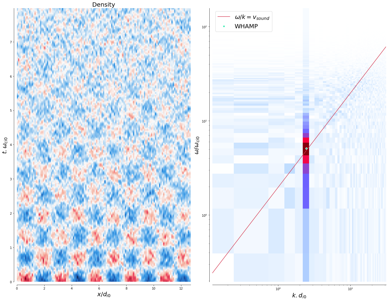
The wavelength is fixed by the box size and fed to WHAMP, obtaining a phase velocity almost equal to the speed of sound, as shown by the white circle in the right-hand plot below, matching the simulated wave.
[3]:
dens_t_s = np.load(f'{path}/products/dens_time_space_rank0.npy')
field_omega_k_spectrum((dens_t_s-np.mean(dens_t_s)), 'Density', mp.dt_low, mp.dx_low, mp, loglog=True, disp_rel='acoustic')
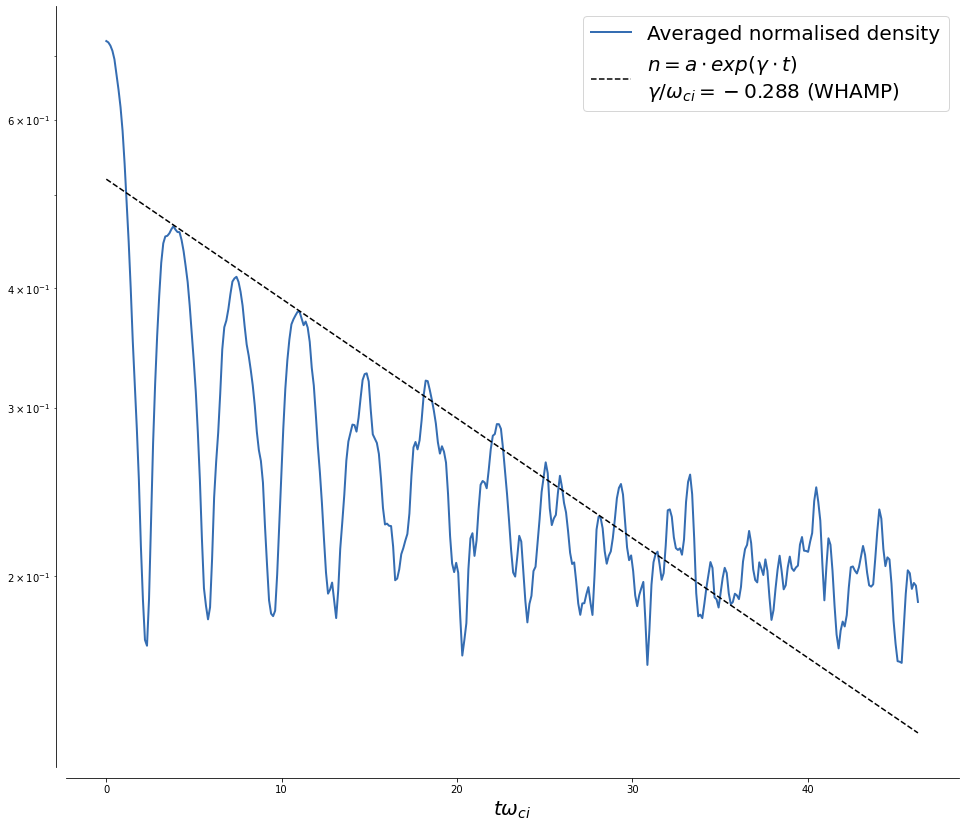
The wave is seen to be damped. We plot now the time evolution of the density at the simulation nodes. The exponential envelop is taken using the WHAMP damping rate.
[6]:
grid_t_low = np.arange(dens_t_s.shape[0])*mp.dt_low

grid_t_low /= mp.omega_ci
gamma = -.0288#*1.2
a = .52#.034#.59

fig, ax = plt.subplots(figsize=(16, 14))

d = np.abs(dens_t_s-1)
d -= np.amin(d, axis=0)
d /= np.amax(d, axis=0)
ax.plot(grid_t_low, np.nanmean(d, axis=1), c=oC.rgb[2], lw=2, label='Averaged normalised density')
ax.plot(grid_t_low, a*np.exp(gamma*grid_t_low), '--k', label='$n = a\cdot exp(\gamma\cdot t)$\n$\gamma/\omega_{ci}=-0.288$ (WHAMP)')


ax.set_xlabel('$t\omega_{ci}$', fontsize=20)
ax.set_yscale('log')
ax.legend(fontsize=20)
oT.set_spines(ax)
plt.savefig('landau.pdf')
plt.show()
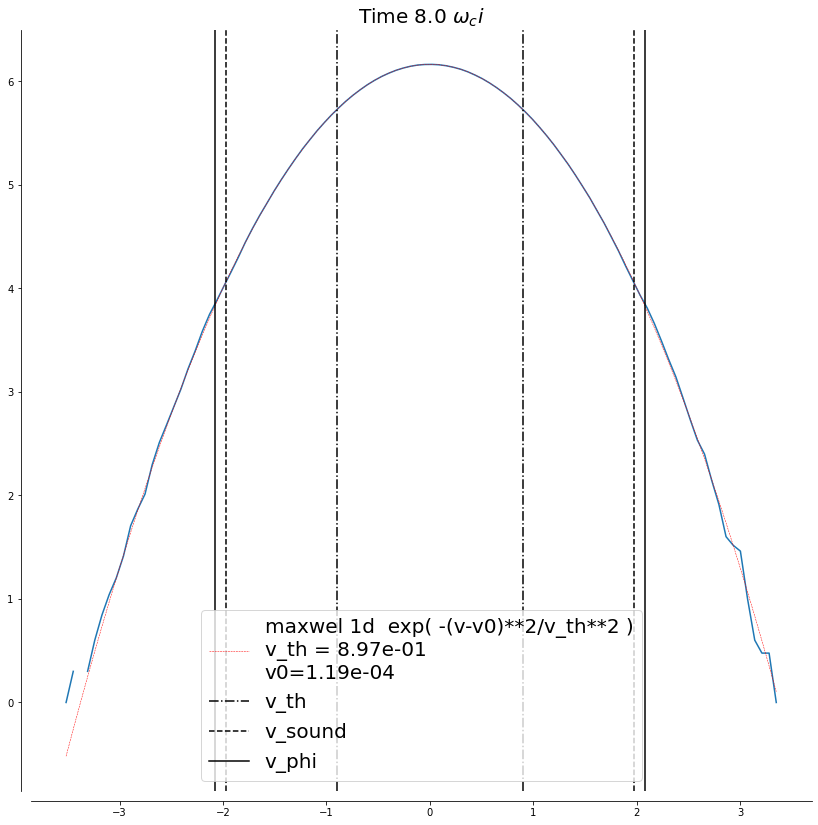
We now look at the signature of this damping on the particle velocity distribution function, identifying the Landau resonant particles around the phase speed of the wave.
[7]:
from scipy.optimize import curve_fit
def maxwellian_1D(v, A, v_th, v0):
    return A * np.exp(-((v-v0)/v_th)**2)
[8]:
ind_it = 4000
p = np.load(f'{path}/products/particles_0_it{ind_it}_rank0.npy').astype(np.float32).T

h_vx, bin_vx = np.histogram(p[2], 100)
centers_vx = .5*(bin_vx[:-1]+bin_vx[1:])

p0 = [np.amax(h_vx), np.var(p[2]), np.average(centers_vx, weights=h_vx)]
p_m, pcov = curve_fit(maxwellian_1D, centers_vx, h_vx)

fig, ax = plt.subplots(figsize=(14, 14))

ax.plot(centers_vx, np.log10(h_vx))#bins)
ax.plot(centers_vx, np.log10(maxwellian_1D(centers_vx, *p_m)),
        '--r', lw=.5, label=f'maxwel 1d  exp( -(v-v0)**2/v_th**2 )\nv_th = {p_m[1]:.2e}\nv0={p_m[2]:.2e}')
v_phi = 5.108/2.454
p_m[1]
ax.axvline(p_m[1], ls='dashdot', c='k')
ax.axvline(-p_m[1], ls='dashdot', c='k', label='v_th')
ax.axvline(mp.v_s/mp.v_A, ls='--', c='k')
ax.axvline(-mp.v_s/mp.v_A, ls='--', c='k', label='v_sound')
ax.axvline(v_phi, c='k')
ax.axvline(-v_phi, c='k', label='v_phi')
ax.legend(fontsize=20)

plt.title(f'Time {ind_it*mp.dt} $\omega_ci$', fontsize=20)
oT.set_spines(ax)
plt.show()
Non-non-linear interaction
If we now increase the initial perturbation amplitude to 0.05 the background density:
[ ]:
mp = menura_param(f'{path}/products')
mp.print_physical_parameters()
mg = menura_grid(f'{path}/products', mp)
[ ]:
dens_t_s = np.load(f'{path}/products/dens_time_space_rank0.npy')
field_omega_k_spectrum((dens_t_s-np.mean(dens_t_s)), 'Density', mp.dt_low, mp.dx_low, mp, loglog=True, disp_rel='acoustic')
[ ]:
grid_t_low = np.arange(dens_t_s.shape[0])*mp.dt_low

grid_t_low /= mp.omega_ci
gamma = -.0288#*np.sqrt(2)
a = .56#.034

fig, ax = plt.subplots(figsize=(16, 14))

d = np.abs(dens_t_s-1)
d -= np.amin(d, axis=0)
d /= np.amax(d, axis=0)
ax.plot(grid_t_low, np.nanmean(d, axis=1), c=oC.rgb[2], lw=2, label='Averaged normalised density')
ax.plot(grid_t_low, a*np.exp(gamma*grid_t_low), '--k', label='$n = a\cdot exp(\gamma\cdot t)$\n$\gamma/\omega_{ci}=-0.288$ (WHAMP)')

ax.set_xlabel('$t\omega_{ci}$', fontsize=20)
ax.set_yscale('log')
ax.legend(fontsize=20)
oT.set_spines(ax)
plt.savefig('landau.pdf')
plt.show()
[ ]:
ind_it = 4000
p = np.load(f'{path}/products_landau/particles_0_{ind}_rank0.npy').astype(np.float32).T

h_vx, bin_vx = np.histogram(p[2], 100)
centers_vx = .5*(bin_vx[:-1]+bin_vx[1:])

p0 = [np.amax(h_vx), np.var(p[2]), np.average(centers_vx, weights=h_vx)]
p_m, pcov = curve_fit(maxwellian_1D, centers_vx, h_vx)

fig, ax = plt.subplots(figsize=(14, 14))

ax.plot(centers_vx, np.log10(h_vx))#bins)
ax.plot(centers_vx, np.log10(maxwellian_1D(centers_vx, *p_m)),
        '--r', lw=.5, label=f'maxwel 1d  exp( -(v-v0)**2/v_th**2 )\nv_th = {p_m[1]:.2e}\nv0={p_m[2]:.2e}')
v_phi = 5.108/2.454
p_m[1]
ax.axvline(p_m[1], ls='dashdot', c='k')
ax.axvline(-p_m[1], ls='dashdot', c='k', label='v_th')
ax.axvline(lp.v_s/lp.v_A, ls='--', c='k')
ax.axvline(-lp.v_s/lp.v_A, ls='--', c='k', label='v_sound')
ax.axvline(v_phi, c='k')
ax.axvline(-v_phi, c='k', label='v_phi')
ax.legend(fontsize=20)

plt.title(f'Time {ind*lp.dt} $\omega_ci$', fontsize=20)
oT.set_spines(ax)
plt.show()